Getting started with colvR

The colvR package provides tools for the analysis of multivariate count data that exhibit both overdispersion and zero-inflation, two common features in ecological and environmental datasets.
In particular, the package makes it possible to impute missing data, to estimate Poisson log-normal models enriched with a latent PCA component, and to optimize model parameters through efficient numerical routines.

library(colvR)
#> 
#> Attaching package: 'colvR'
#> The following object is masked from 'package:stats':
#> 
#>     BIC

General model

We consider a dataset of counts collected at $n$ sites across $p$ years.
Let $Y_{ij}$ denote the number of individuals recorded at site $i \in \{1,\dots,n\}$ and year $j \in \{1,\dots,p\}$.
Each observation is associated with a covariate vector $x_{ij} \in \mathbb{R}^d$.

The full covariate matrix $X \in \mathbb{R}^{np \times d}$ typically combines three types of information:

• Site-level covariates ($R \in \mathbb{R}^{n \times d_1}$): descriptors constant across years (e.g. habitat type, geographic attributes).
  
• Year-level covariates ($C \in \mathbb{R}^{p \times d_2}$): descriptors varying across years but shared across sites (e.g. climate indices, survey effort).
  
• Site–year covariates ($E \in \mathbb{R}^{np \times d_3}$): descriptors specific to each site–year combination (e.g. water level, vegetation cover, observer identity).

These blocks are concatenated into: $$X = [R \otimes \mathbf{1}_p \;\;\; \mathbf{1}_n \otimes C \;\;\; E], \qquad d = d_1 + d_2 + d_3,$$ so that each observation $(i,j)$ is described by a covariate vector $x_{ij}$.

---

The Zero-Inflated Poisson Log-Normal with Probabilistic PCA (ZI-PLN-PCA) model generates abundances in two steps:

1. Presence/absence process $$U_{ij} \sim \text{Bernoulli}\!\left(\pi_{ij}\right), \qquad \pi_{ij} = \frac{1}{1+\exp(-x_{ij}^\top \gamma)},$$ where $U_{ij}=0$ deterministically yields $Y_{ij}=0$.
   The parameter vector $\gamma$ encodes how covariates affect the probability of presence.

2. Abundance process conditional on presence $$Y_{ij} \;\sim\; \text{Poisson}\!\left(\exp(x_{ij}^\top \beta + Z_{ij})\right),$$ where $\beta$ controls the covariate effects on abundance, and $Z_{ij}$ is a latent Gaussian effect.

Each site $i$ is associated with a $q$-dimensional latent vector $$W_i \sim \mathcal{N}(0,I_q), \qquad Z_i = C W_i, \quad C \in \mathbb{R}^{p \times q},$$ so that the covariance structure of the latent effects is $$\Sigma = C C^\top .$$

This low-rank formulation parallels probabilistic PCA and parsimoniously captures correlations between years within the same site.

Example

Data

To illustrate the use of colvR, we rely on the dataset fuligule_milouin provided with the package.
This dataset contains winter count data of the Common Pochard (Aythya ferina), a Palearctic diving duck species.
The counts were collected across multiple wetland sites in North Africa over several years, and the dataset is
characterized by a high proportion of zeros and a substantial amount of missing values — making it a suitable
case study for the zero-inflated Poisson log-normal framework implemented in colvR.

data("fuligule_milouin")
Y <- fuligule_milouin$Y ; X <- fuligule_milouin$X
n <- nrow(Y) ; p <- ncol(Y) ; d <- ncol(X)

cat(mean(is.na(Y)), "is the proportion of missing entries in Y.\n")
#> 0.4443353 is the proportion of missing entries in Y.
cat(mean(Y == 0, na.rm = TRUE), "is the proportion of 0's in Y.\n")
#> 0.6705407 is the proportion of 0's in Y.

Choosing the size of the latent space

An important step in model specification is the choice of the dimension $q$ of the latent space.
The function select_model_bic() can be used to compare models fitted with different values of $q$,
based on the Bayesian Information Criterion (BIC). The selected value corresponds to the latent space
dimension that maximizes the BIC score.

We rely on precomputed BIC values (saved in the package) to keep the vignette fast. If you want to recompute them locally, set Sys.setenv(NOT_CRAN = "true") before knitting.

q_grid <- 1:p

use_precomputed <- !identical(Sys.getenv("NOT_CRAN"), "true")

if (use_precomputed) {
  bics <- readRDS(system.file("extdata", "bics_fuligule.rds", package = "colvR"))
} else {
  bics <- select_model_bic(Y, X, Miss.ZIPLNPCA, q_grid)
  # (Optionnel) sauvegarder à nouveau si vous voulez mettre à jour le package :
  # saveRDS(bics, file = "inst/extdata/bics_fuligule.rds", compress = "xz")
}

# Selected q (robuste aux noms)
q <- if (!is.null(names(bics))) as.integer(names(bics)[which.max(bics)]) else q_grid[which.max(bics)]
q
#> [1] 12

plot(q_grid, as.numeric(bics), type = "b",
     xlab = "Latent dimension q", ylab = "BIC")
# (optionnel) surligner q*
points(q, bics[which.max(bics)], pch = 19, cex = 1.2)
abline(v = q, lty = 2)

Model selection via BIC

Fit

Once the latent dimension $q$ has been chosen, we can fit the model using
the function Miss.ZIPLNPCA(). This function estimates the model parameters
while simultaneously imputing the missing entries in the count matrix Y.

fit <- Miss.ZIPLNPCA(Y, X, q)

The returned object is a list containing:

• the estimated parameters of the model (beta, gamma, C, …),
  
• the variational parameters used for inference,
  
• and the imputed count matrix, where missing values in Y are replaced by their predictions.

This fitted object can then be explored to inspect estimated parameters, check convergence,
and evaluate the quality of imputations.

Confidence interval

Beyond point estimates, colvR also provides tools to quantify uncertainty in the parameters.
The function V_theta() computes an estimate of the covariance matrix of the parameters,
based on the sandwich estimator. Using this, we can derive approximate confidence intervals
for the regression coefficients of both the presence (γ) and the abundance (β) models.

cov <- V_theta(Y, X, fit)
theta <- c(fit$mStep$gamma, fit$mStep$beta)
var <- diag(cov)[1:(2*d)]
Intervals <- IC(theta, var)

We now display the point estimates and 95% confidence intervals for the regression coefficients of the presence model ($\gamma$) and the abundance model ($\beta$).

# Build a compact table of estimates and 95% CIs (no dependency on IC())
se <- sqrt(var)
par_names <- c(paste0("gamma_", seq_len(d)), paste0("beta_", seq_len(d)))
ci_tab <- data.frame(
  param = par_names,
  estimate = theta,
  lo = theta - 1.96 * se,
  hi = theta + 1.96 * se,
  group = rep(c("gamma (presence)", "beta (abundance)"), each = d),
  stringsAsFactors = FALSE
)

# Order for plotting: gamma first, then beta, top-to-bottom
ci_tab$param_pretty <- factor(ci_tab$param, levels = rev(ci_tab$param))

op <- par(mar = c(5, 10, 2, 2))
plot(
  x = ci_tab$estimate, y = as.numeric(ci_tab$param_pretty),
  xlab = "Coefficient (estimate with 95% CI)", ylab = "",
  yaxt = "n", pch = 19, xaxs = "i", col = ifelse(ci_tab$group == "gamma (presence)", "black", "gray30")
)
segments(ci_tab$lo, as.numeric(ci_tab$param_pretty),
         ci_tab$hi, as.numeric(ci_tab$param_pretty),
         lwd = 2, col = ifelse(ci_tab$group == "gamma (presence)", "black", "gray30"))
abline(v = 0, lty = 2)
axis(2, at = seq_along(levels(ci_tab$param_pretty)), labels = levels(ci_tab$param_pretty), las = 1)
legend("bottomright", inset = 0.01, bty = "n",
       legend = c("gamma (presence)", "beta (abundance)"),
       pch = 19, col = c("black", "gray30"))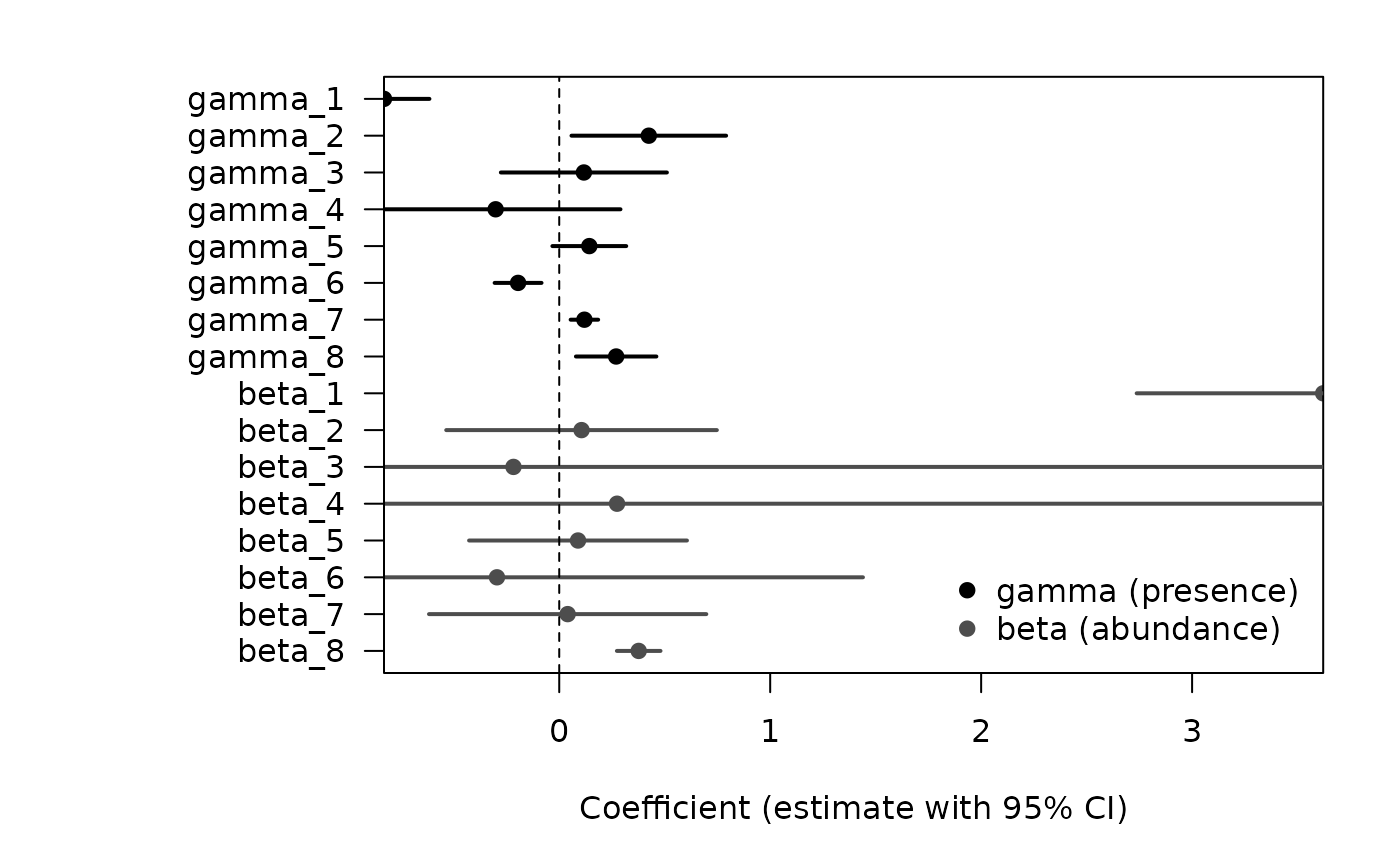

Regression coefficients with 95% confidence intervals

par(op)